TL;DR:

Defintion: P-value is the probability of observing the current or more extreme data conditioned on a true null hypothesis. (key words are highlighted). Note that it is a conditional probability, and it is NOT only about observing the current data, but also more extreme ones.

P-value could be written as

\[\mathrm{Pr}(X \le x|H_0)\]

This is the formula for one-tailed test, and generalizable to the other-tail or two-tail tests. Here, we will focus on one-tail test. $H_0$ means that null hypothesis is being true. In this post, I will use hypothesis as a shorthand for null hypothesis unless noted otherwise.

Note: Usually, an experiment requires p-value to be smaller than a cutoff known as $\alpha$ significance level. Controlling $\alpha$ to be low (e.g. 0.05) is equivalent to keeping specificity high (0.95) as $\alpha + \textsf{specificity} = 1$. If you haven’t thought about $\alpha$ and specificity together before, a related discussion on this topic can be found on stats.exchange.

P-value provides little information about the sensitivity or false discovery rate (FDR) of a test. A somewhat surprising fact is that with a p-value of 0.05, a sensitvity of 0.8, and a prior probability of 0.99 for a null hypothesis being true, FDR could be as high as 0.86. In other words, 0.05 is too generous a cutoff for p-value in general.

Calculation of p-value

I have heard of null-hypothesis testing for a long time, but not until recently, I set out to implement several common hypothesis testing methods (t-test, Mann–Whitney U test, Wilcoxon signed-rank test, Fisher’s exact test) myself, trying to internalize my understanding.

The calculation of a p-value follow a consistent pattern.

First, the data under consideration is summarized with a test statistic. For example, the test statisic is called $Z$ in z-test, $T$ in t-test, $U$ in Mann-Whiteney U test, $W$ in Wilcoxon signed-rank test. In Fisher’s exact test, with the margins fixed, any of the four cell values could be considered a test statistic (ref). In a way, a test statstic could be considered as a single-value representation of the data under consideration.
Then, by locating the observed value of the test statistic in its probability distribution, p-value is obtained by integrating over the area that corresponds to the current statistic value and more extreme ones.

This process would sound familiar if you have conducted t-test before. When I learned t-test for the first time, I was taught to look up a critical value in the t-table instead of computing the p-value directly, which could be difficult without a computer. The critical value is the value of a test static that corresponds to a desired upper bound of p-value (e.g. 0.05, aka significance level, $\alpha$). So even without knowning the exact p-value, by comparing my calculated t value to the critical value, we could know my p-value is above or below $\alpha$.

You may wonder how do we know about the probability distribution of a test statistic. It should have been proved when the testing methods were initially developed. For example, $Z$ follows a normal distribution, $T$ follows a t-distribution. Both $U$ (Mann–Whitney U test) and $W$ (Wilcoxon signed-rank test) follow a normal distribution when the sample size is large, so they essentially become z-test once the statistic is obtained. For Fisher’s exact test, since the probability distribution is discrete, so all probabilities corresponding to the current or more extreme tuplets are calculated and then summed up.

Distribution of p-values under null hypothesis

When the null hypothesis is true, p-value follows a uniform distribution. A brief proof using the universality of uniform distribution is provided below.

Let $P = F(X)$, the cumulative distribution function of $X$. Then, $X = F^{-1}(P)$.

\[\begin{align*} P &= \mathrm{Pr}(X \le x | H_0) \\ &= \mathrm{Pr}(F^{-1}(P) \le x | H_0) \\ &= \mathrm{Pr}(P \le F(x) | H_0) \\ &= \mathrm{Pr}(P \le p | H_0) \end{align*}\]

Therefore, P follows a uniform distribution.

Frequentist interpretation of p-value

We will interpret the p-value from two perspectives, frequentist and Bayesian. Let’s start with the frequentist view.

What does a p-value exactly mean? The definition in the TL;DR section may sound still too abstract, I find it very useful to interpret p-value in the context of a confusion table;thus, it is the frequentist view.

	Condition positive (CP, False null hypotheses)	Condition negative (CN, True null hypotheses)	Row margin	Row metrics
Predicted positive (PP, rejected hypotheses)	True positive (TP)	False positive (FP) Type I error	PP = TP + FP	PPV = TP / PP Positive predictive rate, Precision	FDR = FP / PP False discovery rate
Predicted negative (PN, accepted hypotheses)	False negative (FN) Type II error	True negative (TN)	PN = FN + TN	FOR = FN / PN False omission rate	NPV = TN / PN Negative predictive rate
Column margin	CP = TP + FN	CN = FP + TN
Column metrics	TPR = TP / CP True positive rate, Sensitivity, Recall, Power (1-$\beta$)	FPR = FP / CN False positive rate, $\alpha$ level, significance level
Column metrics	FNR = FN / CP False negative rate, $\beta$ level, operating characteristic	TNR = TN / CN True negative rate, Specificity, confidence level (1-$\alpha$)

The table is adapted from wiki with a more consistent naming and styling convention applied. For example,

All eight metrics are named with three-letter acronyms (TPR, FPR, FNR, TNR, PPV, FDR, FOR, NPV). Their full names, as well as alternative names, are listed below their respective equations. Relatively more well-known metrics are italicized.
All input variables to the equations are named with two letters, and they are colored to be more trackable.
- Marginal sums (CP, CN, PP, PN) are black, while
- the other four key variables (TP, TN, FP, FN) are colored differently.
- As for background color, those with grey background colors are the variables/metrics that the higher, the better. You could see them distributed diagonally.
- Row/Column margins are higlighted in light grey.
- Hovering a cell of interest will related cells, and you shall see the pattern of which metrics are related to which variables. Yellow highlight means variables needed to calculate the metric under cursor. Orange highlight means metrics that use the variable under cursor.
Aside of CP, CN, PP, PN, I also add their respective description in the context of null hypothesis testing.

Insight: If you try to match the definition of p-value that is “the probability of observing the current or more extreme data conditioned on that the null hypothesis being true”, you would focus on the CN column since all hypotheses are true in this column so that it meets the condition. If p-value is less than a cutoff (e.g. significance level, α=0.05), then hypothesis is rejected, which results in a false positive. Therefore a p-value is related to the FPR. To be more concrete, since p-value follows a uniform distribution under true null hypotheses (see derivation above), when you conduct multiple tests, an $\alpha$ portion of those tests would turn out be false positive. Therefore, keeping the $\alpha$ low is equivalent to keeping the specificity high, and an $\alpha$ of 0.05 corresponds to a specificity of 0.95. In other words, FPR = 1 - specificity = $\alpha$.

This post is mostly about single-hypothesis testing (SHT), but here I’d like to put a few notes about p-values in the context of multiple-hypothesis testing (MHT).

While $\alpha$ level in a single hypothesis test can be interpreted as 1 - specificity, it could have a different interpretation in MHT depending on what kind of type I error rate is being controlled, e.g. per-comparison error rate (PCER), family-wise error rate (FWER), or false discovery rate (FDR).
You may have noticed that FDR is also defined in the above table. However, in reality, usually none of TP, TN, FP, FN is known, so they have to be treated as random variables. As a result, FDR could be defined as an expectation instead, i.e. E(FP/PP) as in the famous Benjamini-Hochberg correction method.

Now, we have estabilished the relationship between p-value/$\alpha$ and specificity, does p-value tell us more, for example, sensitivity or false discovery rate (FDR)? Since precision and FDR sum to one, knowing one will get us the other, so we’ll focus only on FDR.

First, since sensitivity and specificity depend on completely different variables (TP and FP vs TN and FN), and these are usually unobserved variables, even if with margins fixed, sensitivity is intractable given specificity. Then, what about FDR? Although FDR and specificity share FP, it is also intractable without further information. As noted in An investigation of the false discovery rate and the misinterpretation of p-values (2014) by David Colquhoun, knowing p-value gets you “nothing whatsoever about the FDR”. This is a bit disappointing, but it is also crucial to keep in mind so as not to over-interpret a p-value.

It turns out there is a simple equation that connects sensitivity, specificity and FDR. Just one more bit of critical information is needed, the prior probability of a hypothesis being false ($\mathrm{Pr}(H_0^C)$ or $r$). In the context of diagnostic method development, the prior probability could be the probability of NOT having a disease in the population. Then, we have

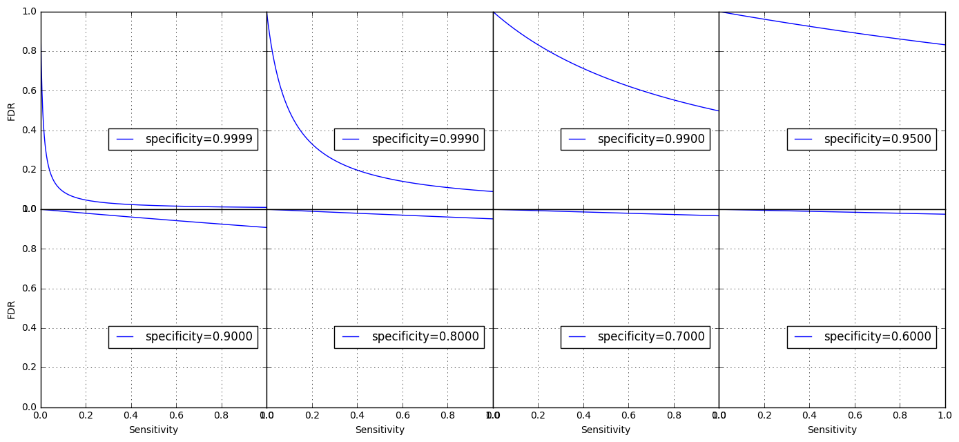
\[\mathsf{FDR} = \frac{N (1 - r) (1 - \mathsf{specificity})}{N(1 - r)(1 - \mathsf{specificity}) + Nr\mathsf{Sensitivity}}\]

$N$ is the population size, which would be cancelled anyway, so we do not need to know its exact value. This relationship is easily verifiable according to the confusion table. Let’s take a concrete example first and then draw a 3D surface to visualize the relationship. Suppose $r=0.01$ (in other words, the disease is rare), specificity is 0.95 (corresponding to the common cutoff of 0.05 for p-value), and sensitivity (power) is 0.80. This is a reasonable setup, not extreme at all, but if you replace the variables with these numbers in the equation, you get a FDR of 0.86, which effectively renders the test method under consideration useless. Remarkably, even when the sensitivity is 1, the FDR is still as high as 0.83. It turns out that increasing sensitivity has a limited effect on the FDR when the $r$ is low and specificity is not high enough (< 0.999), which is seen from the following plots for $r=0.01$ and different specificities.

The surface of FDR ~ sensitivity & specificity is shown below for different $r$ values.

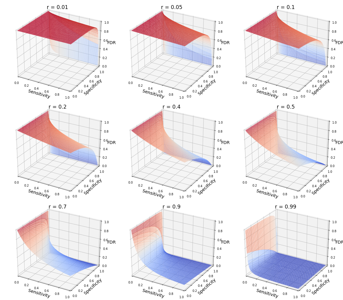
Note when $r = 0.01$ or low in general, FDR is mostly near 1 until specificity becomes extremely high, which explains Colquhoun’s advice that “if you wish to keep your false discovery rate below 5%, you need to … insist on p≤0.001” (i.e. specificity > 0.999). The surface changes as $r$ increases.

The notebook for generating this figure is available at here. In it, I also plotted FDR ~ rate & sensitivity for different specificities.

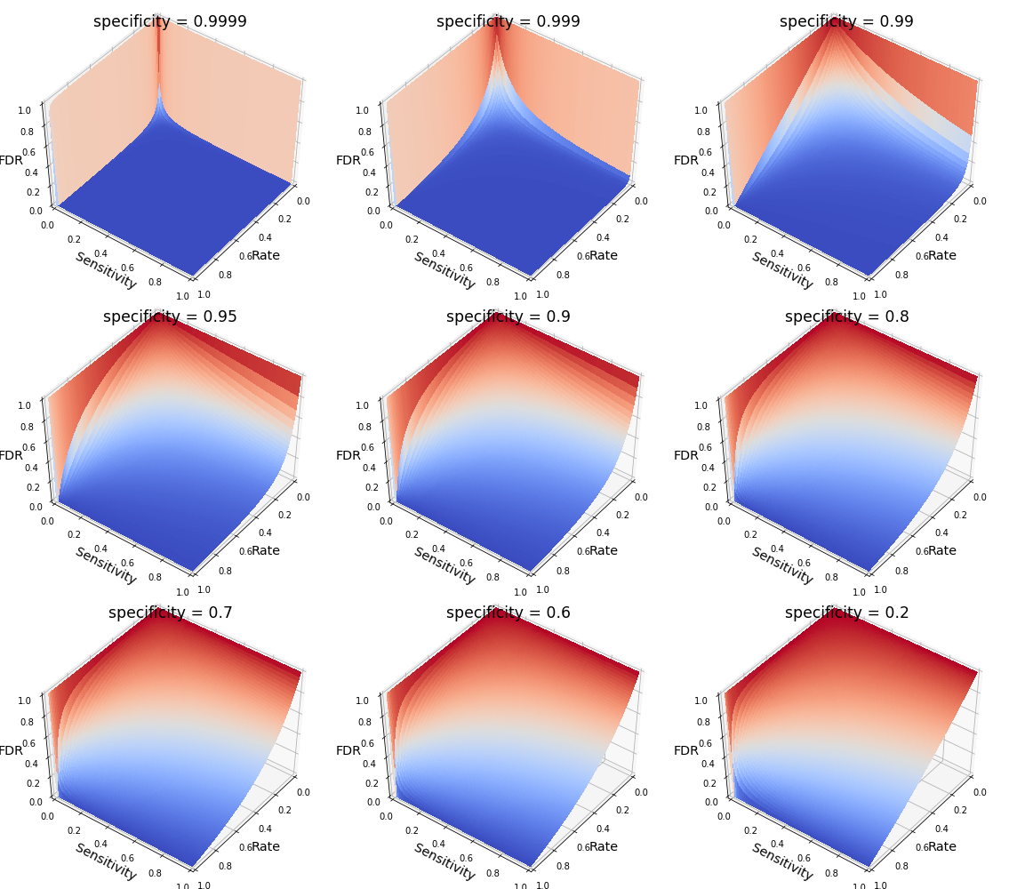
Note when the specificity is very high (0.9999 or 0.9999, in other words, p < 0.0001 or p < 0.001), then the surface is mostly around 0 unless when the rate is extremely low (see the sharp color transitions around the edges, beyond which the FDR shoots up like a rocket).

Bayesian interpretation of p-value

As p-value is a conditional probability, we could write it in terms of Bayes rule, and there comes to be some more insight.

\[\mathrm{Pr}(X \le x | H_0) = \frac{\mathrm{Pr}(H_0 | X \le x)\mathrm{Pr}(X \le x)}{\mathrm{Pr(H_0)}}\]

The left-hand side is the p-value. However, what we usually care the most lies on at the right-hand side that is the probability of null hypothesis being true or false given the test statistic, $\mathrm{Pr}(H_0 | X \le x)$. Unfortunately, without knowing $\mathrm{Pr}(X \le x)$ and $\mathrm{Pr(H_0)}$, we cannot calculate its exact value. Therefore, an important insight from this observation is that rejecting a hypothesis is very different from saying the probability of the hypothesis being true is low or high, or equivalently, the probability of the alternative hypothesis being true is high or low. Actually, they don’t have much to do with each other. Quoting Colquhoun again, rejecting a hypothesis (e.g. p-value < 0.05) simply means it’s worth another look. But you might get a sense already that a cutoff of 0.05 is likely to be really generous, if not too generous.

Summary

If you’ve read the long version, I hope you now have a better sense of the limited information conveyed by a p-value. In summary, a p-value is related to specificity, controlling the p-value to be low is equivalent to keeping the specificity high as $\alpha + \textsf{specificity} = 1$, but it provides little information to the sensitivity or FDR of the test. Importantly, if the prior probability of the hypothesis being false is low which could be common (0.01), then even a very sensitive (e.g. 0.8) and specific (e.g. 0.95) test could still have an unacceptably high FDR (e.g. 0.86). I thought this is the main message conveyed in the seemingly absurdly titled paper Ioannidis JPA (2005) Why Most Published Research Findings Are False. PLoS Med 2(8): e124.. But if you understand how such a high FDR is calculated and the surface plots shown in this post, you may not feel it so absurd anymore.

To me, the widespread of a generally too generous cutoff of 0.05 appears to be an unfortunate accident due to misunderstanding of a p-value. Such generosity explains why some journal went as far as to ban p-values, but in my opinion, it is not that p-value is bad, but more of that a p-value of 0.05 is often too generous a cutoff. Perhaps More importantly, if you insist on having p<0.05, then be conservative with the conclusion, because extraordinary conclusions require extraordinary evidence and the evidence of a p<0.05 is usually not so extraordinary.

This post reflects my current understanding of p-value and null hypothesis testing, if you see any mistake in the post, please let me know by commenting below.